Galaxy-Galaxy Lensing

in this notebook we show how to use glasz to compute \(\Delta \Sigma\) given a halo profile. This is really just a wrapper of a few functions from the pyccl.halos package which can be found here.

# preamble
from __future__ import annotations

import matplotlib.pyplot as plt
import numpy as np
import pyccl as ccl
from init_halo_model import (  # halo model
    a_arr,
    bM,
    cM_relation,
    cosmo,
    hmc,
    hmd,
    k_arr,
    r_arr,
)

import glasz

# CMASS PARAMETERS
z_lens = 0.55  # Mean z for CMASS
a_sf = 1 / (1 + z_lens)

# constituent fractions
fb = cosmo["Omega_b"] / cosmo["Omega_m"]  # Baryon fraction
fc = cosmo["Omega_c"] / cosmo["Omega_m"]  # CDM fraction

# define 2-halo term
xi_mm_2h = glasz.profiles.calc_xi_mm_2h(
    cosmo, hmd, cM_relation, hmc, k_arr, a_arr, r_arr, a_sf
)

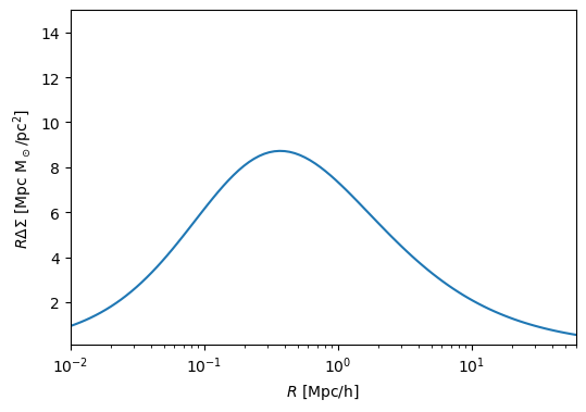
We can simply use the glasz.GGL subpackage to compute \(\Delta \Sigma\) from an NFW profile. To speed up calculation, we make sure to turn on fourier_analytic which will compute the Fourier transform of the NFW profile analytically. The underlying functions used to compute \(\Delta \Sigma\) rely on the pyccl implementation of the fftlog algorithm which is blazingly fast.

We note a subtlety here, the pyccl profiles and glasz.GGL functions assume comoving units without factors of \(h\). If we want to match the observations of Amon & Robertson et al. 2022, we need to properly account for this.

M_halo = 3e13  # solar masses
R = np.geomspace(
    1e-2, 6e1, 100
)  # Mpc/h comoving units (like observations of Amon & Robertson et al. 2022)

prof_nfw = ccl.halos.HaloProfileNFW(
    mass_def=hmd,
    concentration=cM_relation,
    truncated=False,
    cumul2d_analytic=True,
    projected_analytic=True,
    fourier_analytic=True,
)

ds_nfw = (
    glasz.GGL.calc_ds(
        cosmo,
        R / cosmo["h"],  # convert from Mpc/h to Mpc
        M_halo,
        a_sf,
        prof_nfw,
    )
    / cosmo["h"]
)  # convert from Msun/pc^2 to h Msun/pc^2

We can plot it!

f, ax = plt.subplots(1, 1, figsize=(6, 4))
ax.semilogx(R, ds_nfw * R)
ax.set_xlabel(r"$R$ [Mpc/h]")
ax.set_ylabel(r"$R \Delta\Sigma$ [Mpc M$_\odot$/pc$^2$]")
ax.set_ylim(0.1, 15)
ax.set_xlim(1e-2, 6e1)
plt.show()

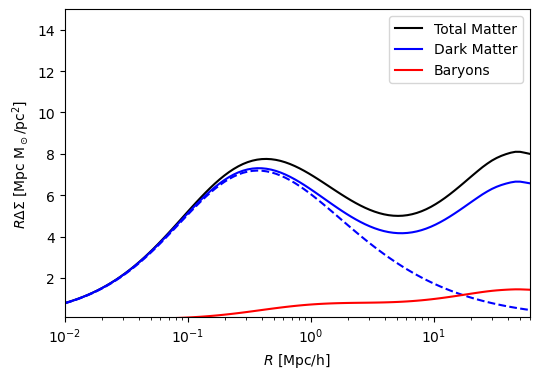
We designed glasz.GGL to take in any pyccl halo profile, one can see this in action below. For more details of what is happening with the creation of these profiles, visit the profiles notebook in the documentation.

# Halo Mass
M_halo = 3e13

# 2-halo Amplitude
A_2h = 0.7

# GNFW Parameters
alpha = 1.0
beta = 3.0
gamma = 0.2
x_c = 0.5

Rb = 10 * (hmd.get_radius(cosmo, M_halo, a_sf) / a_sf)

# COMPUTE GNFW AMPLITUDE
prof_nfw = ccl.halos.HaloProfileNFW(
    mass_def=hmd, concentration=cM_relation, truncated=False, fourier_analytic=True
)

prof_baryons = glasz.profiles.HaloProfileGNFW(
    hmd,
    rho0=1.0,
    alpha=alpha,
    beta=beta,
    gamma=gamma,
    x_c=x_c,
)

prof_baryons.normalize(cosmo, Rb, M_halo, a_sf, prof_nfw)


# COMPUTE 3D DENSITY PROFILES
def rho_2h(r):
    return (
        xi_mm_2h(r)
        * bM(cosmo, M_halo, a_sf)
        * ccl.rho_x(cosmo, a_sf, "matter", is_comoving=True)
        * A_2h
    )


prof_baryons.rho_2h = rho_2h  # add 2-halo term to baryon profile

prof_matter = glasz.profiles.MatterProfile(
    mass_def=hmd, concentration=cM_relation, rho_2h=rho_2h
)

Once the baryon and matter profiles have been created, we can feed them into glasz.GGL.calc_ds like the NFW profile from earlier.

# COMPUTE ΔΣ PROFILE
ds_b = (
    fb
    * glasz.GGL.calc_ds(
        cosmo,
        R / cosmo["h"],  # convert from Mpc/h to Mpc
        M_halo,
        a_sf,
        prof_baryons,
    )
    / cosmo["h"]
)  # convert from Msun/pc^2 to h Msun/pc^2


ds_dm = (
    fc
    * glasz.GGL.calc_ds(
        cosmo,
        R / cosmo["h"],  # convert from Mpc/h to Mpc
        M_halo,
        a_sf,
        prof_matter,
    )
    / cosmo["h"]
)  # convert from Msun/pc^2 to h Msun/pc^2

ds = ds_b + ds_dm

Now we can plot this example!

f, ax = plt.subplots(1, 1, figsize=(6, 4))

ax.semilogx(R, ds * R, color="black", label="Total Matter")

ax.semilogx(R, ds_dm * R, ls="-", color="blue", label="Dark Matter")
ax.semilogx(R, fc * ds_nfw * R, ls="--", color="blue")

ax.semilogx(R, ds_b * R, ls="-", color="red", label="Baryons")

ax.set_xlabel(r"$R$ [Mpc/h]")
ax.set_ylabel(r"$R \Delta\Sigma$ [Mpc M$_\odot$/pc$^2$]")

ax.set_ylim(0.1, 15)
ax.set_xlim(1e-2, 6e1)
ax.legend()
plt.show()