Profiles
This notebook walks through how one can create density profiles which can, in turn, be used to compute either the \(T_{\rm kSZ}\) profile or the \(\Delta \Sigma\) profile.
[2]:
# preamble
from __future__ import annotations

import matplotlib.pyplot as plt
import numpy as np
import pyccl as ccl
from init_halo_model import (  # halo model
    a_arr,
    bM,
    cM_relation,
    cosmo,
    hmc,
    hmd,
    k_arr,
    r_arr,
)

import glasz

# CMASS PARAMETERS
z_lens = 0.55  # Mean z for CMASS
a_sf = 1 / (1 + z_lens)

# constituent fractions
fb = cosmo["Omega_b"] / cosmo["Omega_m"]  # Baryon fraction
fc = cosmo["Omega_c"] / cosmo["Omega_m"]  # CDM fraction

# define 2-halo term
xi_mm_2h = glasz.profiles.calc_xi_mm_2h(
    cosmo, hmd, cM_relation, hmc, k_arr, a_arr, r_arr, a_sf
)
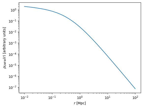
The glasz.profiles subpackage is built on the pyccl.halos package. For this reason, there are several assumptions that go into arguments of these functions. The most important is that all profiles assume comoving units with no factors of \(h\) in units. We can start by making the Generalized NFW (GNFW) profile which is what we use to describe the gas (baryon) density profile. The GNFW profile has the form
which has 5 parameters: the amplitude \(\rho_0\), inner power law slope \(\gamma\) (\(x \ll 1\)), intermediate power law slope \(\alpha\) (\(x \sim 1\)), and the outer power law slope \(\beta\) (\(x \gg 1\)), and the core scale fraction \(x_{\rm c}\).
[12]:
# Halo Mass
M_halo = 3e13

# GNFW Parameters
rho0 = 1.0
alpha = 1.0
beta = 3.0
gamma = 0.2
x_c = 0.5

prof_GNFW = glasz.profiles.HaloProfileGNFW(
    hmd,
    rho0=rho0,
    alpha=alpha,
    beta=beta,
    gamma=gamma,
    x_c=x_c,
)
[33]:
f, ax = plt.subplots(1, 1)
ax.loglog(r_arr, prof_GNFW.real(cosmo, r_arr, M_halo, a_sf))
ax.set_xlabel("$r$ [Mpc]")
ax.set_ylabel(r"$\rho_{\rm GNFW}(r)$ [arbitrary units]")
plt.show()
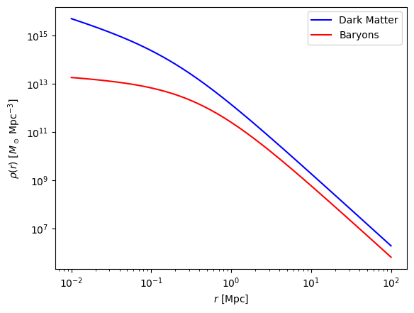
If we want to make this profile physical, we can normalize it relative to an NFW profile such that at the baryon radius \(r_{b}\) the mass enclosed within the GNFW profile is \(f_{\rm b} \times M_{\rm halo}\). In other words
Using this condition, we solve for the baryon density amplitude \(\rho_0\) to get
This removes \(\rho_0\) as a free parameter in the model. We demonstrate how to do this below. For more details
[34]:
Rb = 10 * (hmd.get_radius(cosmo, M_halo, a_sf) / a_sf)

# COMPUTE GNFW AMPLITUDE
prof_nfw = ccl.halos.HaloProfileNFW(
    mass_def=hmd, concentration=cM_relation, truncated=False, fourier_analytic=True
)

prof_baryons = glasz.profiles.HaloProfileGNFW(
    hmd,
    rho0=1.0,
    alpha=alpha,
    beta=beta,
    gamma=gamma,
    x_c=x_c,
)

prof_baryons.normalize(
    cosmo, Rb, M_halo, a_sf, prof_nfw
)  # normalize relative to NFW profile
We can plot this below.
[35]:
f, ax = plt.subplots(1, 1)
ax.loglog(
    r_arr,
    prof_nfw.real(cosmo, r_arr, M_halo, a_sf) * fc,
    label="Dark Matter",
    color="blue",
)  # CDM profile
ax.loglog(
    r_arr,
    prof_baryons.real(cosmo, r_arr, M_halo, a_sf) * fb,
    label="Baryons",
    color="red",
)  # Baryon profile
ax.set_xlabel("$r$ [Mpc]")
ax.set_ylabel(r"$\rho(r)$ [$M_\odot$ Mpc$^{-3}$]")
ax.legend()
plt.show()
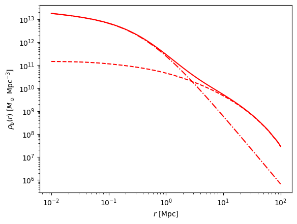
Now that we have the normalization of the GNFW profile to become the baryon (gas) profile. We can also throw in a 2-halo term for each. For more details on how this is done, see the 2-halo section of the documentation.
[36]:
# Amplitude of the 2-halo term
A_2h = 1.0


# Define the 2-halo term from ξ_mm^2h
def rho_2h(r):
    return (
        xi_mm_2h(r)
        * bM(cosmo, M_halo, a_sf)
        * ccl.rho_x(cosmo, a_sf, "matter", is_comoving=True)
        * A_2h
    )


prof_baryons.rho_2h = rho_2h  # add 2-halo term to baryon profile
With this we can plot the baryon (gas) profile. This is what is probed by the \(T_{\rm kSZ}\) measurements.
[38]:
f, ax = plt.subplots(1, 1)
ax.loglog(
    r_arr, prof_baryons.real(cosmo, r_arr, M_halo, a_sf) * fb, color="red"
)  # Baryon profile
ax.loglog(
    r_arr,
    (prof_baryons.real(cosmo, r_arr, M_halo, a_sf) - rho_2h(r_arr)) * fb,
    ls="-.",
    color="red",
)  # 1-halo term
ax.loglog(r_arr, rho_2h(r_arr) * fb, ls="--", color="red")  # 2-halo term
ax.set_xlabel("$r$ [Mpc]")
ax.set_ylabel(r"$\rho_{\rm b}(r)$ [$M_\odot$ Mpc$^{-3}$]")
plt.show()
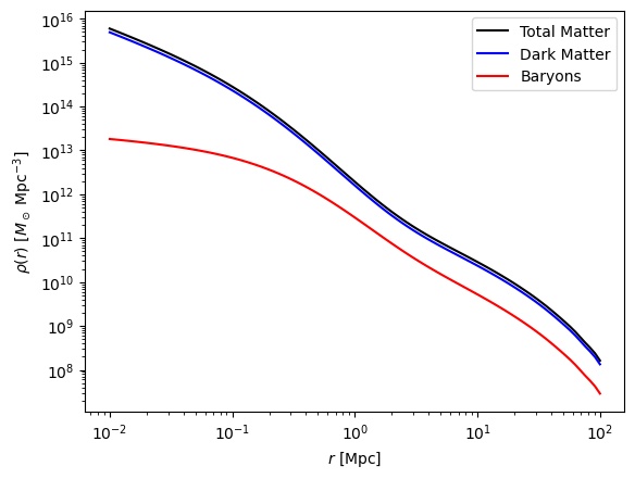
We can finally combine everything to form the matter profile which is what is probed by \(\Delta \Sigma\)
[39]:
prof_matter = glasz.profiles.MatterProfile(
    mass_def=hmd, concentration=cM_relation, rho_2h=rho_2h
)
Lastly, we plot.
[41]:
f, ax = plt.subplots(1, 1)
ax.loglog(
    r_arr,
    prof_matter.real(cosmo, r_arr, M_halo, a_sf),
    color="black",
    label="Total Matter",
)
ax.loglog(
    r_arr,
    (prof_nfw.real(cosmo, r_arr, M_halo, a_sf) + rho_2h(r_arr)) * fc,
    color="blue",
    label="Dark Matter",
)
ax.loglog(
    r_arr,
    (prof_baryons.real(cosmo, r_arr, M_halo, a_sf)) * fb,
    color="red",
    label="Baryons",
)
ax.set_xlabel("$r$ [Mpc]")
ax.set_ylabel(r"$\rho(r)$ [$M_\odot$ Mpc$^{-3}$]")
ax.legend()
plt.show()
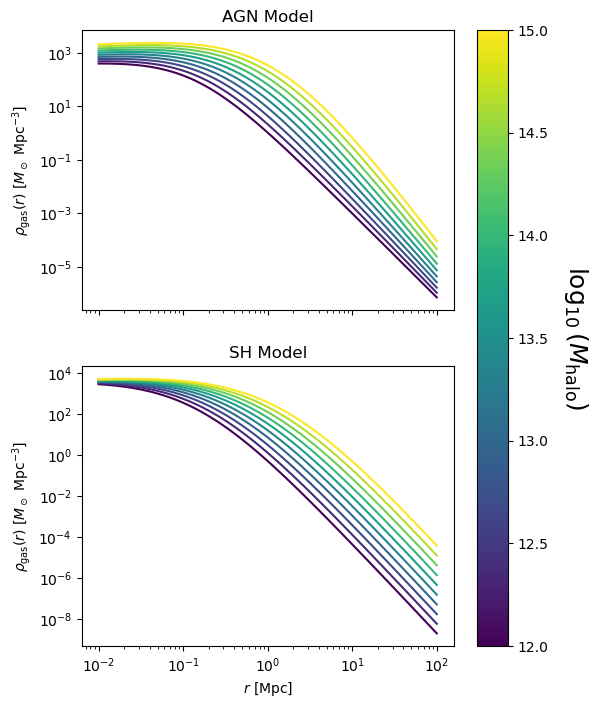
GNFW Parameters as a Function of Mass
In Battaglia et al. 2016, relationships were fit using hydro cosmological simulations to describe \(\alpha\), \(\beta\), and \(\rho_0\) as a function of halo mass and redshift. There are two prescriptions:
“AGN” - Simulations with AGN feedback (strong feedback)
“SH” - Simulations with Adiabatic Cooling (mild feedback)
We have implemented these in glasz.profiles and they can be accessed via
[42]:
profile_gas_AGN = glasz.profiles.HaloProfileGNFW(
    mass_def=hmd,
    feedback_model="AGN",
    truncated=False,
)

profile_gas_SH = glasz.profiles.HaloProfileGNFW(
    mass_def=hmd,
    feedback_model="SH",
    truncated=False,
)
We plot as a function of mass
[65]:
M_arr = np.geomspace(1e12, 1e15, 10)
cmap = plt.cm.viridis
colors = cmap(np.linspace(0, 1, len(M_arr)))

f, axes = plt.subplots(2, 1, figsize=(6, 8), sharex=True)

for i in range(len(M_arr)):
    axes[0].loglog(
        r_arr, profile_gas_AGN.real(cosmo, r_arr, M_arr[i], a_sf), color=colors[i]
    )
    axes[1].loglog(
        r_arr, profile_gas_SH.real(cosmo, r_arr, M_arr[i], a_sf), color=colors[i]
    )

for ax in axes:
    ax.set_ylabel(r"$\rho_{\rm gas}(r)$ [$M_\odot$ Mpc$^{-3}$]")

norm_scaling = plt.cm.colors.Normalize(
    vmin=np.log10(M_arr[0]), vmax=np.log10(M_arr[-1])
)  # set the max and min y value for your cmap
cbar = plt.colorbar(
    plt.cm.ScalarMappable(norm=norm_scaling, cmap=cmap), ax=axes
)  # create color bar object
cbar.set_label(
    r"$\log_{10}(M_{\rm halo})$", rotation=270, labelpad=30, fontsize=18
)  # give cbar a label and rotate it

axes[1].set_xlabel("$r$ [Mpc]")
axes[0].set_title("AGN Model")
axes[1].set_title("SH Model")
# ax.legend()
plt.show()
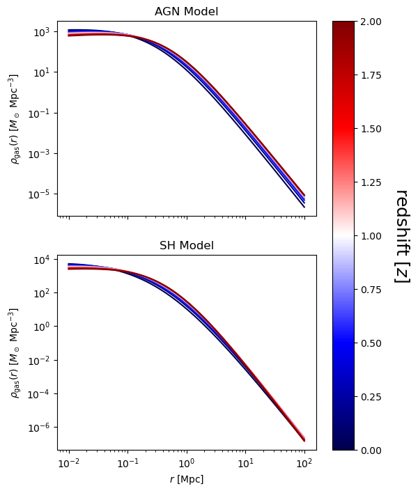
[69]:
z_arr = np.linspace(0, 2, 10)
cmap = plt.cm.seismic
colors = cmap(np.linspace(0, 1, len(z_arr)))

f, axes = plt.subplots(2, 1, figsize=(6, 8), sharex=True)

for i in range(len(M_arr)):
    axes[0].loglog(
        r_arr,
        profile_gas_AGN.real(cosmo, r_arr, M_halo, 1 / (1 + z_arr[i])),
        color=colors[i],
    )
    axes[1].loglog(
        r_arr,
        profile_gas_SH.real(cosmo, r_arr, M_halo, 1 / (1 + z_arr[i])),
        color=colors[i],
    )

for ax in axes:
    ax.set_ylabel(r"$\rho_{\rm gas}(r)$ [$M_\odot$ Mpc$^{-3}$]")

norm_scaling = plt.cm.colors.Normalize(
    vmin=(z_arr[0]), vmax=(z_arr[-1])
)  # set the max and min y value for your cmap
cbar = plt.colorbar(
    plt.cm.ScalarMappable(norm=norm_scaling, cmap=cmap), ax=axes
)  # create color bar object
cbar.set_label(
    r"redshift [$z$]", rotation=270, labelpad=30, fontsize=18
)  # give cbar a label and rotate it

axes[1].set_xlabel("$r$ [Mpc]")
axes[0].set_title("AGN Model")
axes[1].set_title("SH Model")
# ax.legend()
plt.show()
[ ]: